NHL Draft Pick Value (Review)

We all know first round picks are worth more than second round picks and that a #1 pick is worth more than a #4 pick, but by how much?  I’m far from the first person who has tried to answer this question.  In this post we’ll take a look at a few different methods people have tried and the corresponding results.  Will there be a consensus?

In this method, some dedicated plugger must compile a list of all players drafted in a certain period of time and then spend many, many hours assigning subjective values based on their quality according to their own choice of criteria. This is probably the most labor intensive method listed here, by far, but it allows you to use data from players who are still relatively young. For example, Sidney Crosby has not played nearly as many games or scored as many goals as Jarome Iginla, but it’s clear that he should be given a very high value.  

I’m presenting two data sets compiled by two different people:

If a player is good, he’s usually going to play more games in the big league. Exceptions obviously exist.  Many comparatively undistinguished players will have longer careers than Mark Giordano, simply because he took so long to become a NHL regular. However, with a large enough sample size this should be a decent method.  The major downside to this method is that you really need to look at complete careers, so recent draft data cannot be included. Hence, this method might produce results that are somewhat out of date, although whether or not that happens is difficult to determine.

The data set I’m presenting here is:

If a player is good, he’s going to play a lot of minutes. In this method, you find the career total minutes per game that a player has played and then divide it by the average TOI/g that players of his position have played (i.e. Player career TOI/g / Average TOI/g for player position). For this method, you could probably sample half a player’s career and get a good idea of where he stands (I’m not sure if that was done in the data set I’m presenting here).

The data set for this method is:

Obviously, there are many other methods of ranking NHL players. Using possession stats is obviously tempting, but we don’t have adequate historical data to make a decent sample size. Tom Awad once tried to evaluate the success of a team’s draft based on GvT (Goals Versus Threshold), but he didn’t really try to rate the value of various draft positions versus each other, nor did he post data or adequate tables (LINK). As such, this method is not included in the following graphs and is mentioned here for completeness only.  

One method I thought of and haven’t seen used anywhere else is player salary over total league salary for a given year.  If a player scooped up a high percentage of the dollars paid to hockey players in a given year, he was probably pretty good. Unfortunately, I’ve had trouble finding a comprehensive source of NHL salary data that goes back into the 80’s or 90’s, so this will have to wait for another day.  

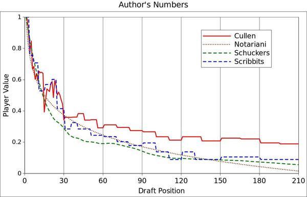
The first plot is simply the data provided by the various sources, normalized so that a number 1 draft pick has a value of 1. A pick with a value of 0.5 (mid first-round) is worth half as much as a #1 overall pick according to this approach. As you would expect, the various methods produce data that is a little bit noisy, although Notarianni provides numbers that appear to have already been put through a logarithmic regression.

To give us a better idea of how these methods compare, I’ve gone ahead and done log regressions for them all, as shown in the following graph. R^2 values for the curves were 0.936, 0.934, 1.00 (because Notarianni only provided fitted numbers), and 0.942 respectively.   On this graph I’ve also included a line from “Eric T” (LINK), which doesn’t aim to represent player value, but rather, trade-value based on actual pick for pick trades. 

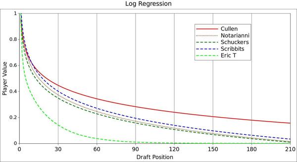
There are some interesting things to note here.  First, the “Eric T” line, based on pick swaps, drops off incredibly fast!  Much faster than any of the other lines presented here.  This may represent the divide between the value of picks and the price.  Alternatively, it may simply be skewed by trades for top 5 picks that don’t follow the overall trends (more on this below). 

Next, Cullen and Notarianni provide very different curves even though they used the same method.  They both use similar sample sizes, although Cullen’s is a bit more recent.  However, the inherent subjectivity of Method #1 is probably a bigger factor.  It looks like Cullen was systematically too mean to the best players and too nice to the awful ones. 

What’s really interesting though, is that Methods #2 (Schuckers) and #3 (Scribbits) agree so well with each other, and with Notarianni as well. Scott Cullen is the only real outlier. When three different methods give similar results it suggests we might be on to something that’s not total horse hockey!

First of all, we’ll disregard the “Eric T” equation since it likely measures something very different from the other curves. Like a naughty little undergrad, I’m going to look the curve that I don’t like (Cullen’s) squarely in the eye and say “To hell with you!”.  I’m tempted to throw Notarianni’s out too, since Method #1 really is subjective, but it agrees so well with Methods #2 and #3 that it doesn’t make much difference. Average those three curves together, and you get the following equation:

Value = -0.1824 ln(draft position) + 0.995  (or 1, if it really bothers you that a #1 overall isn’t valued at 1)

(Note: A power regression might have produced a more appropriate fit.  It does fit Schuckers better.  However, it wouldn’t have fit Notarianni’s at all. A log-fit is acceptable for Schuckers and I wanted to avoid mixing fit types  so as to keep this equation simple.  In future reviews, other fit types should be kept in mind. )

According to this equation, the Flames #4 overall pick is worth 0.75 of the #1 overall pick, which suggests that adding a late second rounder or early third rounder (#61 is worth 0.25) would be a completely fair trade if the Flames wanted to move up.

Dale Tallon would probably not agree with this assessment. 

First of all, market value is more closely related to what buyers are willing to pay rather than actual value (e.g. Monster Cable). Teams are making bonkers offers for the #1 overall pick, so there’s no way a fair trade (based on value) is going to happen.

Second, exceptional individuals have a habit of bucking population trends. While the value equation we’ve found here is probably pretty accurate, on average, it may break down in the top 5 where the truly exceptional individuals are. To put it another way, while the average 1st rounder is probably fairly similar from year to year, the #1 pick is a lot more variable: e.g. Nail Yakupov is no Sidney Crosby!  So salt this sucker well before swallowing!

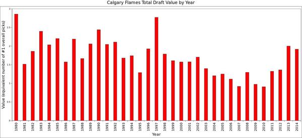
Be honest. The kid in you wants to look under the Flames Christmas tree and see how big the boxes are this year. The above chart adds up the position based value of each draft in the Flames’ history. The average haul got smaller in the 90’s as the league expanded, but 1997 stands out as the biggest draft for the Flames ever in terms of raw materials. Amazingly, 1997’s #6 overall pick never played a single NHL game and the entire 1997 Flames draft class played a total of 81 NHL games. The biggest, spiffiest, shiniest boxes ever put under the Flames tree were entirely full of coal! 

The Flames investment in the draft slowly dropped off year after year from 1997 until 2010, when it finally hit rock-bottom under the shifty, cupboard-raiding fingers of Darryl Sutter. Note that this decline is not the result of an expanding league; the Flames were simply keeping fewer and fewer picks. 2011 and 2012 were better years, thanks to Feaster’s commitment to restock the cupboards, and 2013 was the biggest Flames draft since 1997. In 2014 the Flames may not have as many picks as they did in 2013, but their overall value is nearly the same thanks to the #4 overall pick and two very nice second rounders.

Rest assured, there’s plenty under this year’s tree!